TrustMesh: how we built a real-time fraud brain that thinks in graphs and sequences
A heterogeneous GNN chained into a Transformer, scoring Return-to-Origin risk on millions of daily Cash-on-Delivery orders inside a 50 ms p99 budget.
Originally published on the Meesho engineering blog. Reposted here with the diagrams; the version there is canonical. The underlying paper was accepted at AAAI 2026.
Every day, millions of Cash-on-Delivery orders flow through Meesho. The vast majority are legitimate: a first-time buyer in Patna ordering a kurta, a reseller in Surat stocking up on inventory. But tucked inside that volume is a different kind of order, one that was never meant to be delivered.
The package leaves the warehouse, travels hundreds of kilometres, a delivery attempt is made, and the shipment comes back because the address was fake, the customer refused delivery, or the phone number led nowhere. This is Return-to-Origin, or RTO, and it is one of the most expensive failure modes in Indian e-commerce. Our challenge was to catch it before the package ever left.
Why RTO is a surprisingly hard problem
COD accounts for 60 to 65% of orders in Indian e-commerce, and RTO within COD is the abuse vector that hurts the most, not just in logistics costs but in a cascade of downstream effects on inventory, seller payouts, and customer trust. Global online payment fraud losses are projected to cross $107 billion by 2029, and in the Indian context, LexisNexis estimates that for every ₹1 lost to fraud, businesses absorb a total cost of ₹4 once overheads and chargebacks are included.
The problem is not just one of financial scale. It is one of structural complexity. When we sat down to design a detection system, we identified six distinct failure modes that any serious solution must handle.
Data imbalance. RTO-prone orders are rare, so a model that simply predicts “legitimate” for everything will be right more than 90% of the time and utterly useless in practice.
Evolving fraud. Abusers adapt through bots, synthetic identities, and coordinated collusion, which means the patterns that caught fraud last quarter may not catch it this quarter.
Entity heterogeneity. RTO risk is not localized to a single entity. It spans users, suppliers, products, delivery zones, and device fingerprints, requiring a model that can reason across all of them simultaneously.
Hidden risk, or the “clean profile” problem. A sophisticated abuser does not start out fraudulent. They place several legitimate orders first, building a clean history, and only then exploit it. A model that looks only at a user’s own order history will miss this pattern entirely.
Sparse histories. Many users are new and have only two or three orders in their history, which means sequence-based models that need rich behavioral data will fail exactly when risk assessment matters most.
Temporal volatility. RTO often emerges through a burst, a sudden cluster of returns or refusals, so the temporal shape of behavior matters and not just its aggregate statistics.
No single modality solves all six failure modes, and that is the core insight that led us to build TrustMesh.
The architecture idea: two minds, one model
The fundamental design principle behind TrustMesh is that graph topology and behavioral sequences capture complementary information, and you need both.
A graph tells you who a user is connected to, their structural position in the network of users, suppliers, and shared identifiers. A Transformer sequence model tells you how that user has behaved over time, the pattern of their orders, cancellations, and returns. Neither is sufficient on its own: a Transformer without graph context will miss the user who has a clean personal history but is sharing a device with three known fraudsters, while a graph without sequence context will struggle with temporal bursts from a user who was fine for six months and then suddenly placed twelve RTO orders in ten days.
TrustMesh chains the two together. The GNN runs first, encodes structural context into a dense embedding, and hands it off to the Transformer as just another feature. The Transformer then reasons jointly over topology, static attributes, and behavioural history in a single forward pass.
Stage 1: building the graph
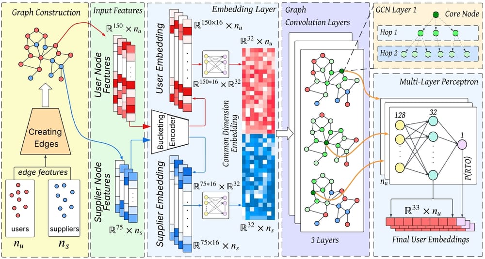
The heterogeneous graph G = (V, E) contains two node types: users (feature vector in ℝ¹⁵⁰) and suppliers (feature vector in ℝ⁷⁵). User features encode ordering frequency, return and cancellation rates, delivery success history, and region-specific behavioral signals. Supplier features capture fulfillment efficiency, dispute rates, and customer interaction patterns.
Three edge types link them across the graph.
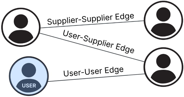
User-user edges are drawn when two users share at least one identity-related attribute such as bank account number, UPI ID, email, phone number, device ID, or Google Advertising ID (GAID). These edges model account duplication and coordinated abuse.
Supplier-supplier edges capture potential collusion between sellers. An edge is instantiated if two suppliers share identifiers like tax registration, bank account, phone, or device ID; if they offer visually similar catalogs measured by cosine similarity of BEiT image embeddings applied to catalog images; or if they serve significantly overlapping user bases.
User-supplier edges represent transactional and identity-based interactions. An edge is added if a user and supplier share identifying attributes or if the user has significant adverse outcomes with that supplier.
This three-way edge structure is important because user-user edges catch fraud rings, supplier-supplier edges catch coordinated seller abuse, and user-supplier edges catch targeting patterns. Any one of them in isolation would miss the other two.
Stage 2: training the GNN
The GNN is a three-layer heterogeneous Graph Convolution network. Before training, node features are bucketized into 20 equal quantile bins and mapped to 16-dimensional embeddings via trainable lookup tables. These are projected to a shared 32-dimensional latent space and then processed through three relation-specific GC layers. After the final layer, an MLP head produces a structural embedding hv in ℝd_gnn for each node.
Training uses binary cross-entropy over labeled “core nodes”, which are users with known RTO outcomes from a 15 to 20 day observation window expanded to six hops of neighborhood context per observation day.
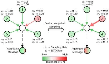
The key training trick is RTO-rate-weighted neighbor sampling. Standard mini-batch sampling on imbalanced graphs tends to undersample the rare but important high-risk neighborhoods, so instead we define an edge-level sampling weight:
w_e = (ω_vi + ε)(ω_vj + ε)
ω_v = (# RTO in last 6 months) / (# orders in last 6 months)
This biases training batches toward RTO-prone neighborhoods, helping the model learn minority-class representations without discarding the majority.
Inference runs daily on a freshly constructed graph built from the preceding six months of transactions, keeping embeddings current as the fraud landscape evolves.
Stage 3: the Transformer
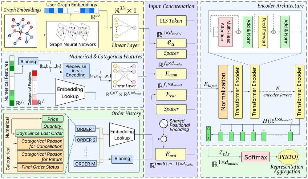
The Transformer module takes four kinds of input and fuses them into a single contextual sequence.
Graph embeddings. The structural embedding hu produced by the GNN is linearly projected into the Transformer’s model dimension d_model, giving every user a learned “topological fingerprint” derived from their graph neighborhood.
Numerical features. Static numerical features such as ordering frequency, historical return rates, and regional signals are encoded using Piecewise Linear Encoding (PLE), a technique that maps each numerical feature into a vector of bin-level activations and then projects it with a learned linear transform. PLE outperforms simple normalization for tabular features, particularly in the presence of long-tailed distributions.
Categorical features. Static categorical features covering user type, preferred language, and preferred search method are embedded via learned lookup tables.
Order history. Each user’s last m ≤ 50 orders are encoded as sequences where each order is a six-dimensional tuple: final status, total price, item quantity, days since placement, cancellation reason, and return reason. Features within each order are embedded independently and then augmented with a shared positional encoding applied uniformly to all six fields of the same order. This “shared positional anchor” is a deliberate design choice that ensures the Transformer treats all fields within a transaction as a single behavioral snapshot rather than independent tokens.
Spacer tokens [S] are inserted between orders to mark transaction boundaries, and the complete input sequence takes the form:
Γ_input = [ [CLS]; γ_u; [S]; Γ_num; Γ_cat; [S]; Γ_ord; [S] ]The [CLS] token’s output representation is used for final classification and in ablation studies it outperformed both average pooling and attention pooling. Loss is weighted binary cross-entropy with class weights inversely proportional to label frequencies, further addressing the imbalance problem.
Does it actually work? Five research questions
Rather than just reporting overall metrics, we structured our evaluation around the five failure modes of RTO detection described earlier.
RQ1: Does TrustMesh outperform baselines?
On our dataset of 10.6M training orders and 1M test orders, TrustMesh outperforms every baseline across tabular, deep learning, transformer-based, graph-based, and unified model categories.
| Architecture | Model | AUCPR | Precision |
|---|---|---|---|
| Tabular | XGBoost | 0.34 | 58.7% |
| DNN | Yuan et al. | 0.30 | 55.3% |
| Transformer | Li et al. 2025 | 0.38 | 61.8% |
| Graph | Best graph baseline | 0.31 | 56.3% |
| Unified | Lin et al. 2024 | 0.45 | 66.9% |
| Unified | TrustMesh | 0.47 | 68.3% |
TrustMesh achieves an AUCPR of 0.47 and 68.3% precision, outperforming the strongest unified baseline by 1.4pp on both metrics. Against XGBoost, the improvement is 9.6pp in precision, which is operationally significant at the scale of millions of daily orders.
RQ2: Does graph context catch fraud rings?
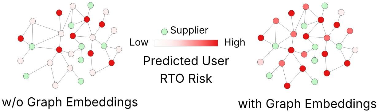
We constructed a cohort of 5,000 users with non-anomalous personal histories but structural links to other users or suppliers via shared attributes. On this cohort, TrustMesh without graph embeddings scores 43 AUCPR and 66.4% precision, while TrustMesh with graph embeddings scores 46 AUCPR and 68.1% precision. The qualitative picture is even clearer: the graph-augmented model exposes dense clusters of interconnected high-risk users and suppliers that the behavior-only variant cannot see at all.
RQ3: Does it catch the “clean profile” abuser?
We tested on 5,000 users with zero prior RTOs or cancellations but structural links to high-risk entities. The behavior-only model scores 27 AUCPR and 58.9% precision, while adding graph embeddings pushes this to 36 AUCPR and 63.4% precision. Multi-hop reasoning through the graph is the only way to surface latent risk that leaves no personal behavioral trace.
RQ4: Does it work for cold-start users?
On a cohort of 5,000 users with four or fewer orders, the model without graph embeddings scores 28 AUCPR and 59.3% precision, while the graph-augmented version reaches 34 AUCPR and 62.5% precision. The GNN compensates for sparse personal history by routing risk signals through the user’s network neighbors.
RQ5: Does it capture temporal volatility?
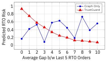
We tested whether TrustMesh assigns higher risk to users whose RTOs cluster in time versus users whose RTOs are evenly spaced, controlling for total count. TrustMesh shows a clear inverse relationship between inter-RTO gap and predicted risk score, while the graph-only baseline shows almost no correlation with temporal clustering.
Deploying at scale: the engineering story
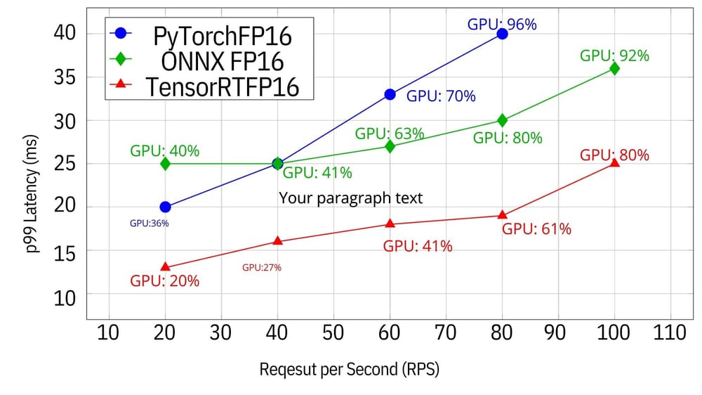
Getting a model to 0.47 AUCPR in a notebook is one thing, and running it on millions of daily orders in under 25 milliseconds is another. The inference stack is built on NVIDIA Triton Inference Server with TensorRT-optimized Transformer models in FP16, which roughly doubles throughput at similar latency compared to a PyTorch FP16 baseline under 80% GPU load.
The p99 latency budget breaks down as: feature store retrieval under 10ms, model inference under 30ms, and an end-to-end p99 latency under 50ms.
The data pipeline. Graph embeddings are refreshed daily from the preceding six months of transactions, while static numerical and categorical features are served from a feature store and order histories are pulled at inference time. The Model Proxy handles routing, batching, and threshold enforcement.
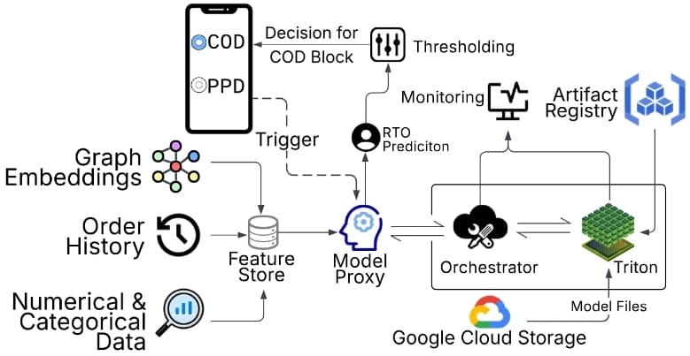
Graph embeddings at inference. The GNN runs as an offline daily batch, producing embeddings for all active users and suppliers that are stored in the feature store and retrieved at online inference time. This decouples the expensive graph computation from the real-time latency budget entirely.
Threshold calibration. Decision thresholds for COD blocking are periodically recalibrated to track the precision-recall tradeoff against evolving business objectives, because the cost of a false positive (blocking a legitimate order) and a false negative (letting an RTO through) changes with operational context.
Model refresh. Retraining is triggered only on statistically significant trend shifts, occurring roughly every 6 to 8 months at a cost of approximately $150 to $200 per cycle, which balances performance stability with operational efficiency. Weekly monitoring of RTO delta, precision, and recall tracks drift between retraining cycles.
What the production data shows
TrustMesh was A/B tested against the incumbent XGBoost model on live traffic, starting at a 5% test and 5% control group and scaling progressively to 20%, 50%, and finally 95% of traffic. The experiment ran for 24 weeks: the first 8 under XGBoost and the following 16 under TrustMesh.
The results held throughout the entire deployment window: a 9.6% absolute precision improvement at fixed recall corresponding to a constant daily COD block rate, an estimated 5pp reduction in operational expenses from reduced RTO, and gains that remained stable over 16 weeks despite traffic and product fluctuations.
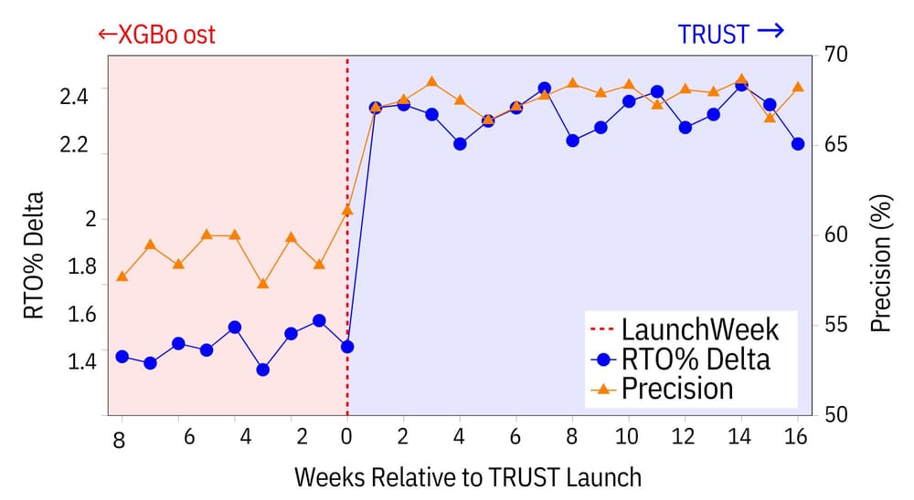
The stability over 16 weeks is the result we are most proud of. It is easy to see a short-term win in an A/B test; it is harder to build a model that continues to beat the baseline as the fraud landscape evolves and seasonal traffic patterns shift.
What we learned
Graph and sequence models are more complementary than competitive. The ablations make this concrete: neither alone achieves what the joint model does, and the failure modes they cover barely overlap. If you are building fraud detection and choosing between GNNs and Transformers, the answer is “yes, and.”
Weighted neighbor sampling matters more than architecture when your graph is imbalanced. We tested multiple GNN variants, but the biggest lift on minority-class recall came from the RTO-rate-weighted sampling strategy, which is a training trick rather than an architecture change.
The “shared positional anchor” for order fields is underrated. Applying a single positional encoding to all features of the same order, rather than per-feature positional encodings, improved empirical performance and reflects a reasonable inductive bias: all features of one transaction should be treated as a coherent snapshot.
TensorRT in production is worth the investment. The throughput gains are real, and at millions of daily requests, the difference between 40 RPS and 80 RPS at p99 under 30ms is an infrastructure cost story and not just a performance footnote.
What’s next
TrustMesh is live and working, but the natural next questions are already on the roadmap. On the graph side, the current schema captures user-user, user-supplier, and supplier-supplier relationships, and there are other entity types such as delivery zone networks, device fingerprint clusters, and product category graphs that could enrich the topology considerably.
On the interpretability side, a precision gain is useful but a model that can explain why it flagged an order is more useful still. We are exploring causal approaches that can separate structural association from genuine risk factors, which matters both for interpretability and for robustness against adversarial adaptation. Sophisticated fraudsters who learn that TrustMesh exists will adapt their behavior, and preemptively hardening the model against adversarial graph manipulation such as deliberately breaking the identity links that TrustMesh relies on is an open problem worth solving before it becomes urgent.
This paper was accepted at AAAI 2026 and the full technical details are available there. If you are building fraud or abuse detection at scale and want to go deeper on the GNN architecture, the sampling strategy, the deployment stack, or the A/B test methodology, we are happy to discuss.
Research by Rithvik Y, Bhavuk Singhal, Shubham Jain, Akshat Garg, Karan Tanwar, Anshu Aditya, Debashis Mukherjee and Debdoot Mukherjee — Meesho Data Science team. Diagrams © Meesho, reproduced from the original post.
All writing